Exercise 3: Performing Analysis in AGOL
Overview
In this exercise, we will explore the analytical capabilities of ArcGIS Online. Our context will be to build a dataset used to develop a species distribution model for some salamanders. Specifically, we want to generate a new set of attributes for locations where a few salamander species have been observed in south central Texas. We will derive these attribute through various spatial analysis operations executed entirely in ArcGIS Online.
Learning outcomes
In doing this exercise, you will gain experience with the following techniques and concepts:
- Importing MS Excel files into hosted feature service layers
- Creating a classic web map from your feature layers
- Searching for and adding additional layers to your web map
- Running vector analyses in AGOL
- Running raster analyses in AGOL
- Creating and executing Raster Functions in AGOL.
- Managing the inputs and outputs of these tools within AGOL
- Evaluate the pros and cons of performing analyses in AGOL relative to desktop GIS
Tasks
- Obtain and upload the salamander point locations to AGOL
- Build a web map for analysis
- “Enrich” the salamander points
- Spatial Joins in AGOL - Intersect
- Spatial Joins in AGOL - Nearest Feature
- Extracting raster values for each salamander location
- Extracting raster values near a subset of salamander locations
- Compute percent forest cover upstream of each Species 2 point
- Recap
Additional Resources
- Documentation: https://doc.arcgis.com/en/arcgis-online/analyze/perform-analysis.htm
- More lessons: https://learn.arcgis.com/en/paths/data-analysis/
- Sneak peak of what’s coming soon: Slide Deck | Recording
Procedure
1. Obtain and upload the salamander point locations to AGOL
The first step is to add our own data to AGOL so that we can include it in our analysis.
NOTE: The data provided for this analysis, while extracted from publicly available literature, has not been expressly verified and should not be distributed outside of this lesson. They are for demonstration purposes only.
- Create a new folder in your AGOL account to hold your project files.
- Download the MS Excel file of salamander points here (via Sakai).
- Add the data to your AGOL account as a hosted feature layer into your new project folder. Remember to add your NetID or some other unique identifier to your object names.
2. Build a web map for analysis
Analysis is done in the AGOL web map; this has to be the “Web Map Classic” option as only that version is equipped with the analytical tools. We’ll create our map from our new salamander point feature layer, and then add a few raster layers:
-
Open your Salamander feature layer in a new classic map viewer. Rename your salamander points layer to “
Salamander points” [Optional] Symbolize this layer so each species of salamander is shown differently. -
In the map viewer, browse the Living Atlas (hint: use the “
Add ▼” tab) for the USA Soils Map Units feature layer. Add this feature layer to your map.
-
In the map viewer, add the USA NLCD image service layer from the Living Atlas.
This image layer is actually a composite of several years worth of NLCD data.
- Click on the map and scroll through the results; there should be 5 years of data.
- Configure the popup for this layer to include
{StartYear}and then click on the map again. You can now see the year that the land cover value corresponds to. - In the next step, we’ll lock in the latest year of data: 2017
-
Filter the USA NLCD Land cover for the latest (2017) land cover dataset:
- Click on the filter icon (the funnel) associated with the layer.
- Apply the query: “Start Year is 2017”. The image service is now only associated with the 2017 land cover data.
-
Search for and add the “Ground Surface Elevation - 30m” image service layer from the Living Atlas.
-
Finally, search ArcGIS Online for “
3d78674c1bc0488c8060ec30c4eccabe” and add the result to your map. (This is the item ID for the National Hydrographic Dataset for SE Texas.)
-
Return to your map and arrange the layers so that the salamander points are on top, all other layers are turned off, and the map is zoomed to the extent of your salamander points.
-
Save your map to the folder containing your salamander points.
3. “Enrich” the salamander points
While it’s unlikely that you’d use demographic data for a species distribution model, we’ll take this opportunity to explore a useful AGOL resource called “Enrichment”, where you can extract data on a wide variety of subject fields for areas intersecting or nearby features you specify.
-
Open the Enrich Layer tool:
From the “Analysis” tab, expand the “Data Enrichment” menu (found within the “Feature Analysis” section) to find the “Enrich Layer” tool. When the tool opens, ensure that theSalamander Pointsis the layer to enrich. -
Select the variables with which we want to enrich our data:
Click the “Select Variables” button to explore the variables you can use to enrich your data. Familiarize yourself with the interface and groupings of data: not only the topics displayed by icons, but the source options in the dropdown menus in the upper right.-
Find the Landscape Variables (Set the source as “United States” and the select “Landscape”)
-
Click the button to show all landscape variables.
-
Select:
Percent of Wetlands (NLCD),Mean Water Table Depth Annual MinimumandPercent of Open Water (NVC Subclass),
then click “Apply”.
-
- Now we must define the area surrounding our locations for which we will summarize our selected variables.
- Select a straight-line distance of 1 km.
- Keep the box for
Return result as bounding areasunchecked.
-
Next, we set our output names and run our analysis.
- Recall that names in AGOL must be unique, so append your outputs with your NetID…
- Be sure that
Use current map extentis unselected. - Have a look at the number of credits enriching your data will consume.
- Run the analysis.
- Finally, tidy and review the output.
- Rename the resulting feature in your web map, something like “Enriched Points (1km)”. Save your map.
- Display the feature layer and click on one of the features to reveal its popup.
- Also, have a look at the feature layer’s attribute table.
- Symbolize the features on the “% Wetlands (NLCD)” attribute. Do you see a pattern?
More about data enrichment can be found here: https://doc.arcgis.com/en/esri-demographics/latest/reference/data-allocation-method.htm.
Some questions to consider when using these data:
- How reliable are the sources?
- How are data allocated to the features and distances you provide?
- What is the “best available apportionment method”?
4. Spatial Joins in AGOL - Intersect
- First, let’s limit our analysis area to save a few credits and speed up processing time:
In the location search box enter “Lost Maples State Park, Vanderpool, TX” to zoom to that area. You should have 4 salamander points in view. (Note that two are very close to each other…)
Tip: consider adding a bookmark for this extent… - Now we’ll attach the Soils Map Unit data to these salamander point features.
- Navigate back to the Feature Analysis toolset menu (where you found the Data Enrichment tool).
- Find and execute the appropriate tool to join the USA Soils Map Unit attributes to the Species 2 point intersecting it. Be sure to keep the analysis constrained to the display extent.
- Rename the output layer in your map view something useful and sensible. Then save your map.
- Check the output: does this appear useful for the task at hand?
5. Spatial Joins in AGOL - Nearest Feature
- Keeping the extent as the zoom to the Lost Maples State Park, select the Find Nearest tool to find the single nearest NHD flowline feature to each of the Salamander points. (Limit the range to 250m.)
- Rename your output layer in your map and examine its attributes.
6. Extracting raster values for each salamander location
- Zoom your map back to the extent of all the salamander points.
- In the Raster Analysis menu, select the Sample tool from the Manage Data section.
- Select the rasters you want to sample (Ground Surface Elevation - 30m and USA NLCD Land Cover).
- Select the location layer (our salamander points).
- Set the output to be a table.
- Ensure to set the analysis to be constrained by the extent and run the analysis.
- View the results. Are the as expected?
7. Extracting raster values near a subset of salamander locations
- Create a copy of your Salamander Points layer, renaming the copy “Species 2 points”
- Filter the records in this new layer for “Species is sp2”. (You should have 6 points in the resulting layer.)
- Zoom to the features in the new feature layer.
- Use the appropriate tool to buffer each Sp2 point a distance of 2km.
- Use the appropriate raster analysis tool to compute a table listing the mean elevation within each of these 2km buffer features.
8. Compute percent forest cover upstream of each Species 2 point
This is our most complex analysis because it requires several steps. First, we need to compute the area upstream of each salamander point. We can do that fairly easily using AGOL’s Watershed tool. But then, to compute the percent forest within each of these watersheds, we need to first convert our NLCD dataset into a forest/non-forest binary raster, and then compute the mean value of all pixels falling within each of these watershed areas.
If we were to do this analysis in ArcGIS Pro, we could perhaps use the Tabulate Area tool to compute the area of each land cover within the different watersheds. However, this tool is not [yet?] available in AGOL. Also, this tool would not work if we had overlapping watershed polygons. So instead, we can compute zonal stats on binary rasters to get the proportion of individual land cover categories.
We could create our forest/non-forest raster using the Remap tool, but we will explore the more powerful Raster Function Editor.
-
Find and execute the appropriate tool to compute watersheds upstream of each species 2 point. (Set the search distance to 250 m.)
→ We could create our forest/non-forest raster using the Remap tool, but we will explore the more powerful Raster Function Editor.
-
In the Raster Analysis settings menu, set the Processing Extent to the same as the watersheds layer and the Snap Raster to the NLCD dataset
-
From the Raster Analysis menu, select the Raster Function Editor button (
 ).
). -
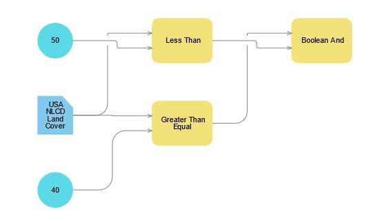
Create a Raster Function that assigns all forest pixels (values 40 thru 49) a value of 1 and everything else to 0.
- Creates a binary output of all NLCD pixels greater than or equal to 40;
- Creates a second binary output of all NLCD pixels less than 50;
- Combines the above two rasters using a Boolean And.
This should appear as below:
-
Save this raster function as “Extract-forest-from-NLCD-
" to your project folder in AGOL. -
Back in the Raster Analysis menu, select Browse Raster Function Templates (
 ), locate the template you just created, and run it.
 -
Compute the zonal mean of the forest binary within each watershed.
Recap
You’ve successfully created a number of feature layers and tables listing new attributes linked to our initial salamander observation locations. These include both vector and raster overlay functions as well as operations to compute buffer and upstream distances relative to our points.
Having completed similar tasks using desktop GIS, you can now compare and contrast the two approaches.
- What are the pros and cons of doing this analysis in AGOL as compared to ArcGIS Pro?
- Did analysis in AGOL meet your expectations (whatever those might have been…)? Keep in mind the analyses you did not execute in this particular assignment…
- Are there features you especially liked or disliked in executing analyses in AGOL?
What’s next…
- We will examine how a similar analysis is executed via a coding platform, both one that uses ArcGIS Online resources (via the ArcGIS API for Python) and one that uses application programming interfaces (APIs) linked to other web-based resources.